Standard Operating Procedure (SOP)
CF-SOP-001 | ChromatographyForge Operation: Explanation of Each Function
1. Document Control
| SOP Number | CF-SOP-001 |
| Title | ChromatographyForge Operation: Explanation of Each Function |
| Version | 1.1 |
| Effective Date | August 19, 2026 |
| Review Date | August 19, 2027 |
| Supersedes | Version 1.0 |
| Department | Analytical Development / QC |
| System | ChromatographyForge |
| GxP Impact | Yes (Data handling, method-development documentation, report generation) |
2. Purpose
Define and explain each major ChromatographyForge function, provide illustrated operational checks, and outline how an analyst establishes a development model from scratch during routine use. The procedure supports consistent operation and data-integrity controls aligned to cGMP expectations.
3. Scope
This SOP applies to all authorized personnel using ChromatographyForge for day-to-day chromatographic model setup, method development, data review, prediction analysis, and report generation in regulated or quality-controlled environments.
4. References
- 21 CFR Parts 210 and 211 (Current Good Manufacturing Practice)
- 21 CFR Part 11 (Electronic Records; Electronic Signatures)
- EU GMP Annex 11 (Computerized Systems)
- ALCOA+ Data Integrity Principles (Attributable, Legible, Contemporaneous, Original, Accurate, Complete, Consistent, Enduring, Available)
- Internal policy: Laboratory Data Governance and Computerized Systems Access Control
- ChromatographyForge Tutorial 002: Iterative Method Development from a Starting Analytical Method
- SOP-ANALYTICAL-014: Site analytical method-development procedure (where applicable)
5. Definitions
| Term | Definition |
|---|---|
| Condition | An independent variable in the method (for example flow, temperature, or pH). |
| Initial Condition | Baseline value used as the reference state for prediction calculations. |
| Target Condition | Desired method value used to project retention time shifts and chromatographic behavior. |
| Development Model | The set of peak-specific condition/retention-time observations and fitted relationships used to predict retention behaviour at trial conditions. |
| Data Point | One experimentally observed condition value and retention time associated with a named peak and condition. |
| Retention Time | Retention time in minutes. |
| Critical Pair | A pair of peaks requiring resolution control for method suitability. |
6. Roles and Responsibilities
| Role | Responsibilities |
|---|---|
| Analyst | Enter data accurately, execute workflows per SOP, review outputs, and retain records. |
| Reviewer / Supervisor | Verify data quality, confirm parameter appropriateness, and approve generated reports. |
| System Administrator | Manage user accounts, role permissions, and system-level settings in accordance with access-control procedures. |
| QA | Audit SOP adherence, data integrity controls, and deviation/CAPA documentation. |
7. Procedure: ChromatographyForge Functions
Global Functions7.1 Header and Project Controls
- Project Name/Status: Identifies current work context.
- New Project: Starts a new workspace.
- Save to Session / Load from Session: Stores/restores active data from browser session storage.
- Download Project / Upload Project: Exports/imports project data file for controlled sharing and archival.
- Recent Projects: Opens recent project list for controlled recall.
cGMP expectation: Ensure correct project name and analyst attribution before data entry.

7.2 Quick Data Input
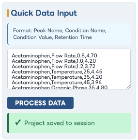
Function: Bulk entry area for four-field records in this format: Peak Name, Condition Name, Condition Value, Retention Time.
Use: Rapid import of experimental points gathered from lab runs.
Control: Use Process Data and verify status message confirms successful processing.
7.3 Initial Conditions
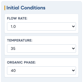
Function: Baseline selectors per condition.
Use: Sets reference values against which target-driven changes are calculated.
7.4 Target Conditions
Function: Numeric endpoint inputs per condition.
Use: Predicts retention time and chromatogram behavior for intended method settings.

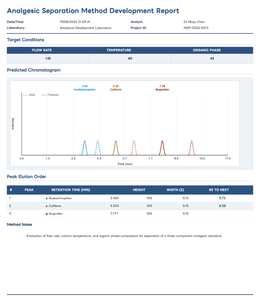
7.5 Predicted Chromatography Panel
- View / Run: Select full run, zoomed peaks, or a custom range and define the displayed run time.
- Overlay / Compare: Display mode toggle for interpretation.
- Auto-fit / Save PNG: Fit the view to the current peaks or export the displayed chromatogram as an image.
- Y Scale: Changes vertical display amplification without changing predicted retention time.
- Initial / Fill / Width follows zoom: Shows baseline positions, fills peak areas, and controls apparent width during zooming.
- Separate / Merged: Draws individual peaks or a combined envelope. Merge threshold, Components, and Valley drops control how overlapping peaks are represented.
- Baseline offset / Noise: Adds a visual baseline position and deterministic noise for realistic presentation.
- Integration controls: Shows integration limits, end ticks, colour, window width, and optional shaded area.
Use: Evaluate predicted separation and elution behavior.
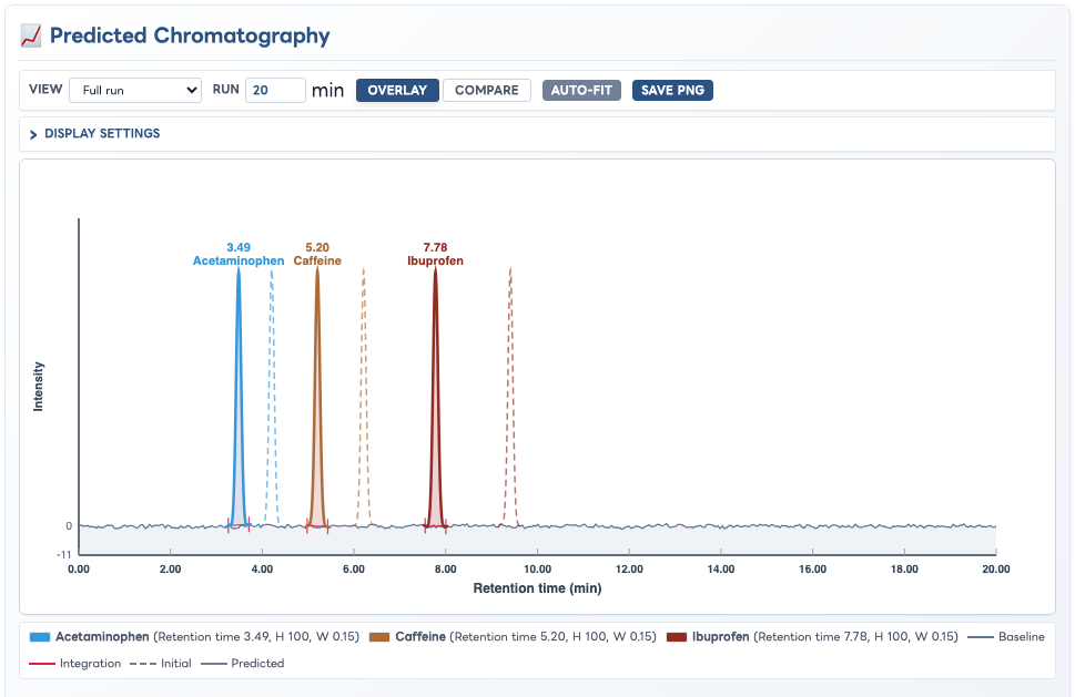
Initial is enabled. The legend identifies peak colour, predicted retention time, height, and width.Interpretation: Use the numerical results and resolution values for decisions; use the chart as a visual aid.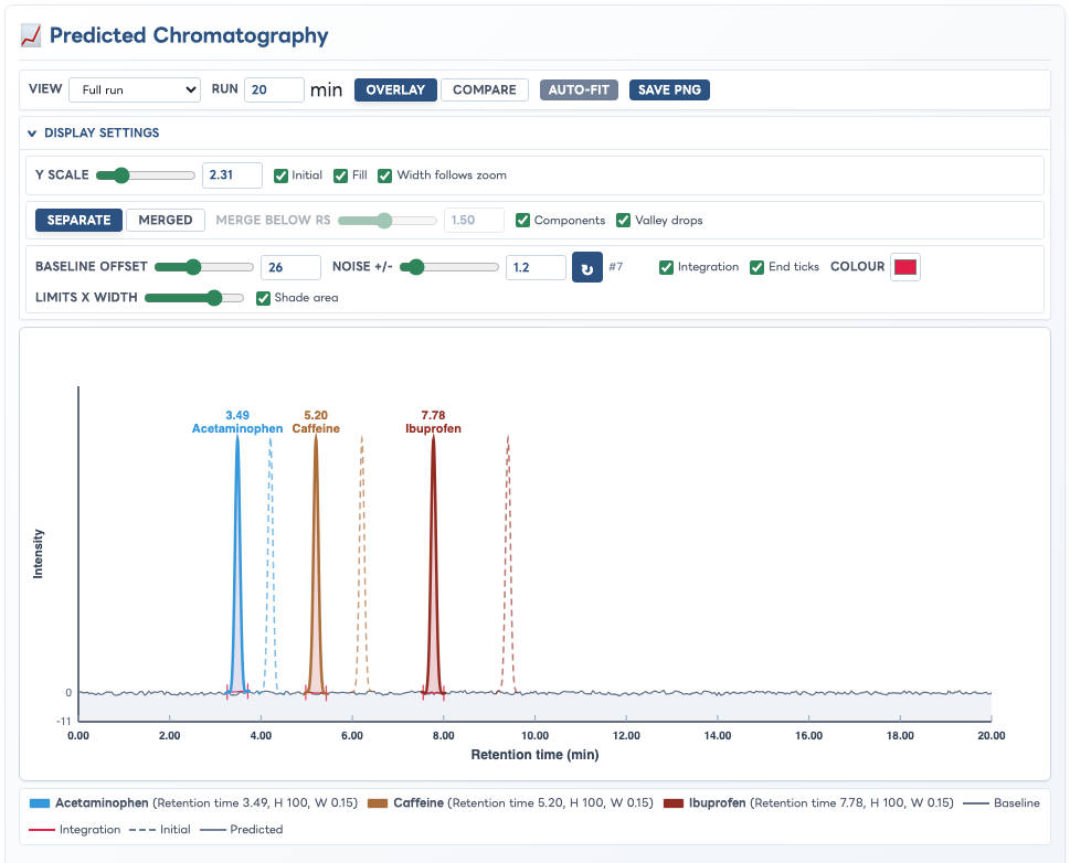
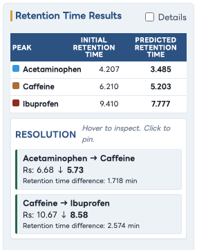
7.6 Retention Time Results and Resolution
Function: Table of initial and predicted retention time values, optional detailed contributions, and resolution metrics.
Use: Supports pass/fail assessment against method performance expectations.
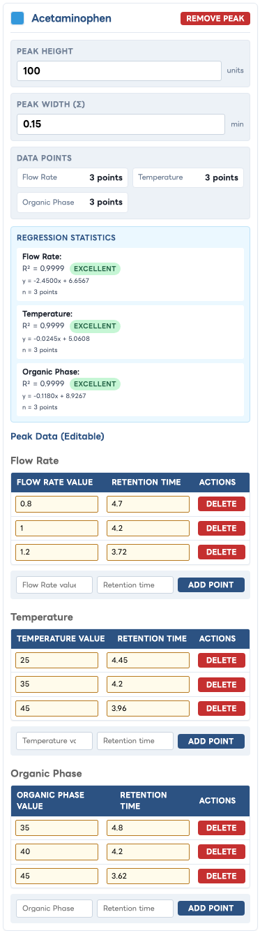
7.7 Peaks Grid and Peak Cards
- Add Peak: Creates a new analyte peak object.
- Peak Properties: Peak height and width tuning inputs.
- Regression Statistics: Displays per-condition fit quality (R², slope, intercept, point count).
- Editable Data Tables: Add/edit/delete data points by condition.
- Color Picker: Assigns peak display color for charts and legends.
Use: Maintain analyte-specific data quality and modeling performance.
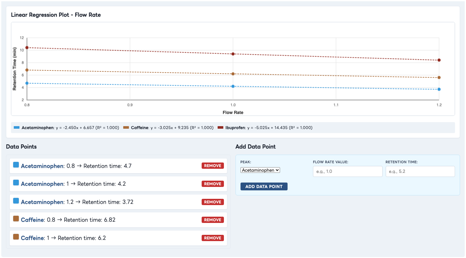
7.8 Add Condition and Condition Workspace
- Add Condition: Adds a new independent variable with baseline value.
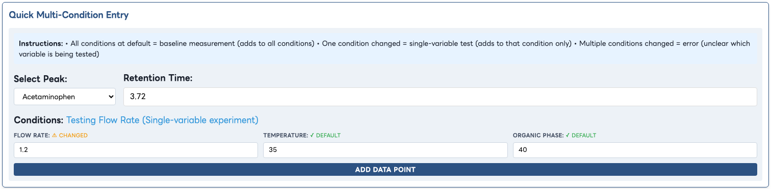
- Quick Multi-Condition Entry: Guided entry mode enforcing baseline/single-variable logic.
- Nested Condition Tabs: Condition-specific graph, data list, and add-point form.
- Linear Regression Plot: Visual fit per peak for selected condition.
Use: Build robust condition-response data for predictive accuracy.
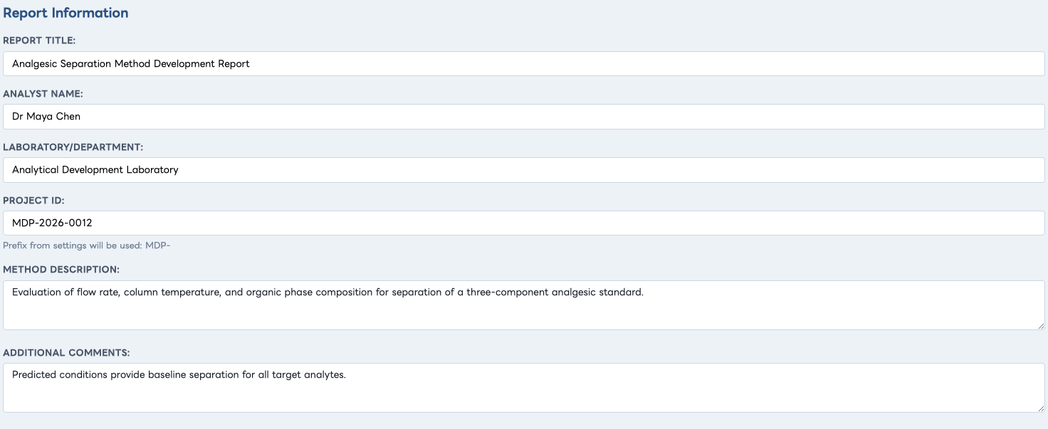
7.9 Report Setup and Output
- Report Information: Title, analyst, department, project ID, description, comments.
- Include Options: Controls report sections (conditions, chromatogram, elution order, resolution, statistics, method development, raw data).
- Method Development Options: Variation levels and design type (full/reduced runs).
- Generate / Print / Download: Creates finalized report and export outputs.
Use: Produce controlled documentation for technical review and archival.
7.10 Application Settings
- Settings File Management: Export/import settings JSON and template.
- Company/Lab Information: Logo and organization metadata.
- Default Report Information: Standard analyst/department/prefix/notes values.
- Report Defaults: Default inclusion checkboxes for generated reports.
- GMP Compliance Settings: Regulatory standard, SOP reference, quality-system reference.
Use: Standardize output, branding, and compliance metadata across users.
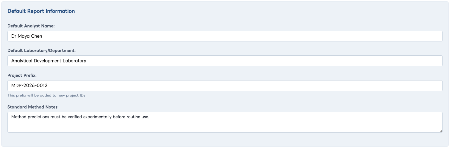
MDP-2026-0012.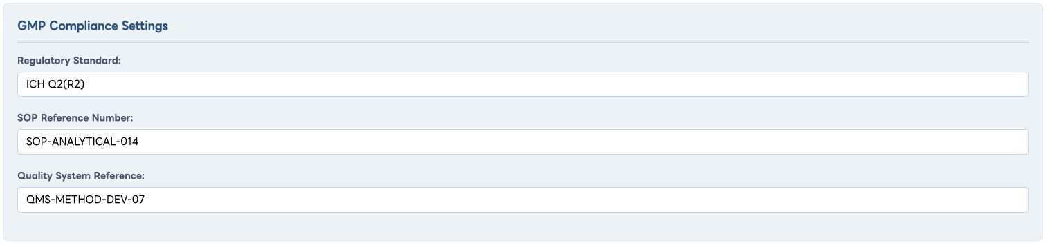
SOP-ANALYTICAL-014 reference, and quality-system reference before controlled reporting.8. Data Integrity and cGMP Controls
- Use unique user credentials; do not share accounts.
- Confirm project identity before entering or modifying data.
- Enter source data contemporaneously and verify numeric accuracy before processing.
- Document corrections with rationale in laboratory records when data are edited or deleted.
- Generate and retain report outputs as part of the controlled study record.
- Follow site procedures for backup, retention, and restricted access.
9. Deviations and Incident Handling
- If incorrect data were processed, stop further reporting and document a deviation.
- Reconstruct corrected dataset from source records and repeat analysis under supervision.
- Escalate software malfunction, access-control issues, or data-integrity concerns to QA and System Administration.
10. Records to Retain
| Record | Minimum Retention Expectation | Owner |
|---|---|---|
| Project data files (.hplc or session export equivalent) | Per site record-retention policy | Analyst / Department |
| Generated reports (print/PDF) | Per approved study or validation record plan | Analyst / Reviewer |
| Settings snapshots (if used) | Retain with report package when settings affect interpretation | Analyst |
| Deviation/CAPA records | Per quality-system retention requirements | QA |
11. Annex A: Function-to-Control Mapping
| Function | Primary Use | Critical Check | Record Evidence |
|---|---|---|---|
| Quick Data Input | Bulk source-data entry | Format and numeric validation | Processed status and saved project snapshot |
| Initial/Target Conditions | Baseline vs target comparison | Scientifically justified values | Report conditions table |
| Chromatogram | Visual prediction review | Critical-pair behavior and peak overlap risk | Report chromatogram image |
| Retention Time Results / Resolution | Numeric suitability assessment | Meets pre-defined acceptance criteria | Report tables and reviewer sign-off |
| Peaks/Conditions Editing | Model refinement | Changes justified from source data | Updated project file and notebook entry |
| Report Generation | Controlled output documentation | Correct options and metadata selected | Final report output (PDF/print) |
12. Annex B: Daily Use Case - Set Up a Development Model from Scratch
This outline shows the normal analyst sequence for creating a new model from experimental measurements. It uses the fictional project illustrated in Figures 1–13. Adapt analytes, variables, ranges, and acceptance criteria to the approved development protocol.
| Example item | Value |
|---|---|
| Project | MDP-2026-0012 - Analgesic Separation Optimisation |
| Peaks | Acetaminophen, Caffeine, Ibuprofen |
| Independent variables | Flow Rate, Temperature, Organic Phase |
| Baseline | Flow Rate 1.00; Temperature 35; Organic Phase 40 |
| Trial target | Flow Rate 1.10; Temperature 40; Organic Phase 43 |
| Illustrative checks | At least three justified points per peak/condition fit; preferred R² ≥ 0.95; protocol-defined critical-pair Rs (commonly ≥ 1.5) |
Define the Development Question
- State the intended separation objective and identify critical analytes or peak pairs.
- Select independent variables supported by the development protocol, such as flow rate, temperature, pH, or organic-phase proportion.
- Define experimentally safe ranges and pre-approved decision criteria before modelling.
- Ensure original chromatograms, integration results, run conditions, and sample identifiers are available as attributable source records.
Output: a documented modelling plan specifying peaks, variables, ranges, baseline, and acceptance criteria.
Create and Identify the Project
- Sign in with the assigned account and confirm the displayed identity.
- Select New Project, enter
Analgesic Separation Optimisation, and associate it with project IDMDP-2026-0012in the laboratory record. - Confirm the project header and status as shown in Figure 1.
- Save to session once so a recoverable working state exists.
Analgesic Separation Optimisation, the saved status, and the signed-in fictional analyst before entering development data.Enter the First Experimental Dataset - Select an Entry Route
Route A - Quick Data Input (bulk entry)
Format every record as Peak Name, Condition Name, Condition Value, Retention Time. The following dataset reproduces the illustrated three-peak, three-variable model.
Show the 27-line example dataset
Acetaminophen,Flow Rate,0.8,4.70
Acetaminophen,Flow Rate,1.0,4.20
Acetaminophen,Flow Rate,1.2,3.72
Acetaminophen,Temperature,25,4.45
Acetaminophen,Temperature,35,4.20
Acetaminophen,Temperature,45,3.96
Acetaminophen,Organic Phase,35,4.80
Acetaminophen,Organic Phase,40,4.20
Acetaminophen,Organic Phase,45,3.62
Caffeine,Flow Rate,0.8,6.82
Caffeine,Flow Rate,1.0,6.20
Caffeine,Flow Rate,1.2,5.61
Caffeine,Temperature,25,6.55
Caffeine,Temperature,35,6.20
Caffeine,Temperature,45,5.87
Caffeine,Organic Phase,35,7.10
Caffeine,Organic Phase,40,6.20
Caffeine,Organic Phase,45,5.32
Ibuprofen,Flow Rate,0.8,10.42
Ibuprofen,Flow Rate,1.0,9.40
Ibuprofen,Flow Rate,1.2,8.41
Ibuprofen,Temperature,25,9.86
Ibuprofen,Temperature,35,9.40
Ibuprofen,Temperature,45,8.95
Ibuprofen,Organic Phase,35,10.92
Ibuprofen,Organic Phase,40,9.40
Ibuprofen,Organic Phase,45,7.91
- Paste the records into Quick Data Input (Figure 2) and select Process Data.
- Confirm that 27 points were processed and that three peaks and three conditions appear.
- Verify representative values against source results. Investigate parsing warnings, negative values, missing combinations, or transcription discrepancies before proceeding.
Route B - Peaks Management (manual per-peak entry)
Use this route when results are being transcribed a point at a time or when the analyst wants to review each peak record as it is assembled.
- In a new project, open Conditions & Data and select + Add Condition three times. Create Flow Rate with baseline 1.0, Temperature with baseline 35, and Organic Phase with baseline 40.
- Open Peaks Management and select + Add Peak three times. Create Acetaminophen, Caffeine, and Ibuprofen.
- Keep Show Details enabled. In each peak card, locate the required condition table, enter the condition value and measured retention time in the Add Point row, and select Add Point.
- The card refreshes after each addition. Return to the relevant peak and condition before entering the next pair.
- Use the following map to reproduce the same 27 records:
| Peak card | Condition table | Condition value → retention time entries |
|---|---|---|
| Acetaminophen | Flow Rate | 0.8 → 4.70; 1.0 → 4.20; 1.2 → 3.72 |
| Acetaminophen | Temperature | 25 → 4.45; 35 → 4.20; 45 → 3.96 |
| Acetaminophen | Organic Phase | 35 → 4.80; 40 → 4.20; 45 → 3.62 |
| Caffeine | Flow Rate | 0.8 → 6.82; 1.0 → 6.20; 1.2 → 5.61 |
| Caffeine | Temperature | 25 → 6.55; 35 → 6.20; 45 → 5.87 |
| Caffeine | Organic Phase | 35 → 7.10; 40 → 6.20; 45 → 5.32 |
| Ibuprofen | Flow Rate | 0.8 → 10.42; 1.0 → 9.40; 1.2 → 8.41 |
| Ibuprofen | Temperature | 25 → 9.86; 35 → 9.40; 45 → 8.95 |
| Ibuprofen | Organic Phase | 35 → 10.92; 40 → 9.40; 45 → 7.91 |

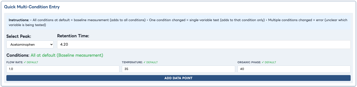
Route C - Quick Multi-Condition Entry (experiment-by-experiment entry)
Use this route when entering results in experimental order. Work by condition state: set the experimental conditions, then record the observed retention time for every peak at that state before moving to the next condition. This example uses a one-factor-at-a-time study, so each non-baseline state differs from baseline in exactly one variable.
- Start from a fresh project and create the same three conditions and three peaks described in Route B.
- Work down the condition-state table below. For each row, establish the displayed Flow Rate, Temperature, and Organic Phase values, then enter the three retention times from left to right.
- At a condition state, select Acetaminophen, enter its RT, and select Add Data Point. After the form refreshes, restore the same condition state, select Caffeine, and add its RT. Repeat for Ibuprofen.
- Complete all three peaks at the current condition state before advancing to the next row. The peak selector identifies which observed peak the RT belongs to; it does not define the order of the workflow.
| Condition state | Flow Rate | Temperature | Organic Phase | Acetaminophen RT | Caffeine RT | Ibuprofen RT |
|---|---|---|---|---|---|---|
| Baseline | 1.0 | 35 | 40 | 4.20 | 6.20 | 9.40 |
| Flow Rate - upper | 1.2 | 35 | 40 | 3.72 | 5.61 | 8.41 |
| Flow Rate - lower | 0.8 | 35 | 40 | 4.70 | 6.82 | 10.42 |
| Temperature - upper | 1.0 | 45 | 40 | 3.96 | 5.87 | 8.95 |
| Temperature - lower | 1.0 | 25 | 40 | 4.45 | 6.55 | 9.86 |
| Organic Phase - upper | 1.0 | 35 | 45 | 3.62 | 5.32 | 7.91 |
| Organic Phase - lower | 1.0 | 35 | 35 | 4.80 | 7.10 | 10.92 |
- For the baseline row, all inputs must show ✓ Default. Each of its three additions records that peak's baseline RT in all three condition models, producing nine underlying condition-specific points.
- For every other row, change only the emphasized input. The other two inputs must show ✓ Default, and the mode message must identify a Single-variable experiment. Each addition is recorded only against the changed condition.
- Enter the upper row before the lower row for each condition. While initially seeding the range, this keeps the intended baseline as the middle/default value.
- After all seven condition states are complete, confirm that 21 Add Data Point actions have produced 27 condition-specific points: three values for every peak/condition combination.
Output: a populated model with three observations for every peak/condition combination.
Set the Baseline and Trial Target
- Set Initial Conditions to Flow Rate 1.00, Temperature 35, and Organic Phase 40 (Figure 3).
- Set Target Conditions to Flow Rate 1.10, Temperature 40, and Organic Phase 43 (Figure 4).
- Confirm the application recalculates without an error and the target values fall within the studied ranges.
Output: a defined reference state and a scientifically plausible trial method.
Review Model Quality and the Prediction
- Open Peaks Management and confirm each peak card contains three points for every condition (Figure 8).
- Review slope direction, point count, and R². Inspect condition plots for unexpected trends or outliers (Figure 9).
- Return to Overview and inspect predicted retention times and all resolution pairs (Figures 5 and 7).
- Use Display Settings only to clarify presentation (Figure 6); do not treat visual amplification, noise, fill, or merged rendering as a change in model performance.
- For the illustrated target, confirm predicted retention times of approximately 3.485, 5.203, and 7.777 minutes and resolution above the illustrative 1.5 threshold.

Output: a documented decision to accept the trial target for experimental testing or to continue refinement.
Refine with Additional Experiments When Required
- If fit or separation is inadequate, identify the variable and range requiring more evidence.
- Perform the new experiment under the approved protocol and retain its original record.
- Add a baseline point or a single-variable point through Conditions & Data. Change only one condition from baseline when using Quick Multi-Condition Entry.
- Re-check the affected regression, all predicted retention times, and resolution after the addition.
- Never remove a valid but inconvenient point solely to improve R²; investigate and document the scientific basis for any exclusion.
Generate, Review, and Archive the Result
- Complete report metadata using the project ID and analyst identity (Figure 10).
- Select the report sections required by the protocol. For technical review, normally include target conditions, chromatogram, elution order, resolution, statistics, method-development conditions, and raw points.
- Generate the report, review every page and optional section, and regenerate after any model change (Figure 11).
- Save to session, download the
.hplcproject, and export the reviewed report according to the site record-retention procedure. - Record the conclusion, experimental follow-up, filename/location, and reviewer disposition in the laboratory record.
12.1 Routine Decision Guide
| Observed state | Required action | Record expectation |
|---|---|---|
| Input parsing warning or incorrect count | Stop, reconcile format and source values, then reprocess. | Correction documented in the contemporaneous record. |
| Weak fit, implausible trend, or insufficient points | Check transcription and source integration; add justified experiments if required. | Investigation rationale and added run identifiers. |
| Target outside studied range | Gather bracketing measurements or select an in-range target. | Protocol justification and supporting experiments. |
| Resolution fails the approved criterion | Change a justified target variable or extend the development design. | Decision rationale and next experiment plan. |
| All criteria met | Experimentally verify the proposed condition, then report and archive. | Project export, report, verification data, and review approval. |
13. Training Requirement
Users shall be trained on this SOP before independent use of ChromatographyForge for GMP-relevant activities. Training completion shall be documented in the site training system.
14. Revision History
| Version | Effective Date | Summary of Change | Author |
|---|---|---|---|
| 1.1 | August 19, 2026 | Added controlled interface figures, expanded function annotations and Display Settings guidance, and added an illustrated routine model-from-scratch use case covering bulk, per-peak, and multi-condition data-entry routes. | ________________ |
| 1.0 | March 1, 2026 | Initial issue. | ________________ |
15. Approval Signatures
| Role | Name / Signature | Date |
|---|---|---|
| Prepared By | ||
| Reviewed By | ||
| Approved By (QA) |
Controlled copy becomes effective only after required approvals are completed.