ChromatographyForge Tutorial 002
Iterative Method Development from a Starting Analytical Method
A novice-friendly worked example that starts with one problematic method, uses Report Generation to recommend the first experiments, feeds measured results into a model, and repeats the cycle until an optimised condition and a defensible operating range can be investigated.
Welcome
This is a learning guide, not a controlled SOP. At the beginning you possess only a starting method and one chromatogram. You do not yet have a response model or a set of screened results. ChromatographyForge first helps you create an experimental plan; only measured results from that plan are then used to build the model.
What you will learn
- Enter a handed-over method as the initial model centre.
- Generate the first one-factor-at-a-time development plan and data-collection sheet.
- Perform the proposed runs and enter only experimentally observed retention times.
- Use the resulting response model to select a more promising condition.
- Centre another development round on that candidate and repeat the evidence cycle.
- Use iterative results to propose - and experimentally challenge - an operating range.
Your starting brief: one method with a problem
Your supervisor supplies the following fictional analgesic method and its latest reviewed chromatogram. No screening work has yet been performed.
| Item | Information available at the start |
|---|---|
| Project | MDP-2026-0012 - Analgesic Separation Optimisation |
| Analytes | Acetaminophen, Caffeine, and Ibuprofen |
| Initial method | Flow Rate 1.00 mL/min; Column Temperature 35 °C; Organic Phase 40% |
| Observed RTs | Acetaminophen 4.20 min; Caffeine 4.50 min; Ibuprofen 9.40 min |
| Observed issue | Acetaminophen/Caffeine is the critical pair; the supplied chromatogram reports Rs approximately 1.0, below the illustrative requirement of 1.5. |
| Development aim | Improve the critical-pair separation while avoiding an unnecessarily long method; preserve peak identity and elution order. |
Define the development problem
Goal: turn the supplied chromatogram into a development question before asking the software for experiments.
- Confirm the peak identities and the reported critical-pair resolution from the source chromatogram.
- Record the initial settings, column, mobile phases, sample information, instrument, and other fixed method parameters.
- Define the acceptance criteria. This tutorial uses critical-pair Rs ≥ 1.5, preserved peak order, and a preference for an earlier final peak.
- Identify hard experimental limits before reviewing generated runs: instrument pressure, column temperature, solvent compatibility, analyte stability, and any protocol-defined boundaries.
Create the project and enter only the initial condition
Goal: establish the handed-over method as the centre from which Report Generation will recommend experiments.
2.1 Create an identifiable project
- Sign in, select New Project, and name it
Analgesic Initial Method Development. - Associate project ID
MDP-2026-0012-R1with the first round in your laboratory record. - Select Save to Session and confirm the correct user, project name, and saved status.


2.2 Create the baseline scaffold
- Open Conditions & Data and add Flow Rate with baseline 1.0, Temperature with baseline 35, and Organic Phase with baseline 40.
- Open Peaks Management and add Acetaminophen, Caffeine, and Ibuprofen.
- Check every spelling and baseline before entering results.


2.3 Enter the starting chromatogram
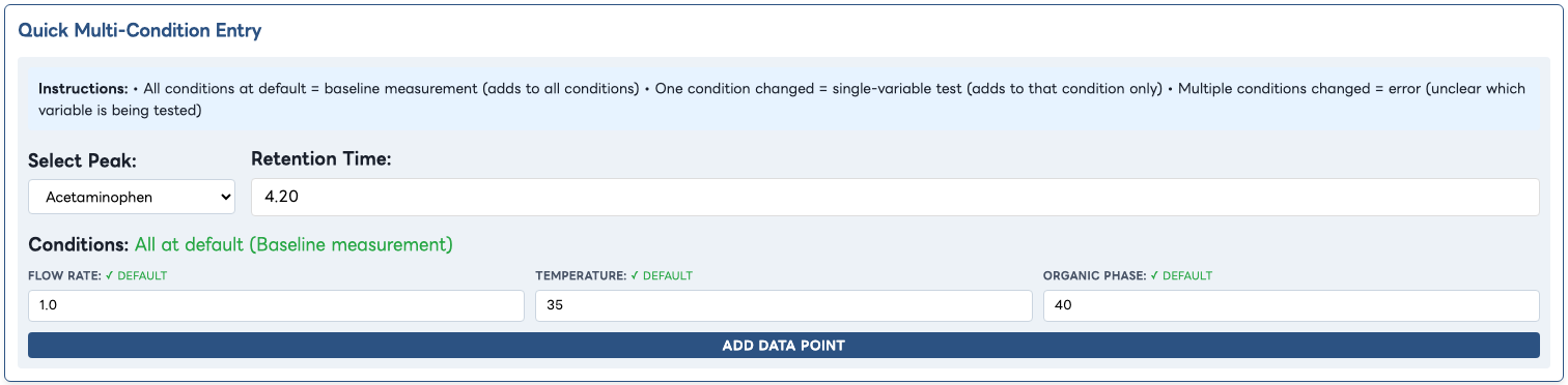
In Quick Multi-Condition Entry, leave every condition at Default. Add the three observed RTs one peak at a time:
| Condition state | Acetaminophen RT | Caffeine RT | Ibuprofen RT |
|---|---|---|---|
| Flow 1.0; Temperature 35; Organic 40 | 4.20 | 4.50 | 9.40 |
Generate the first development plan
Goal: use the initial method as the target centre and obtain a practical data-collection plan from Report Generation.
- On Overview, confirm the target values remain Flow Rate 1.0, Temperature 35, and Organic Phase 40 - the method you currently know.
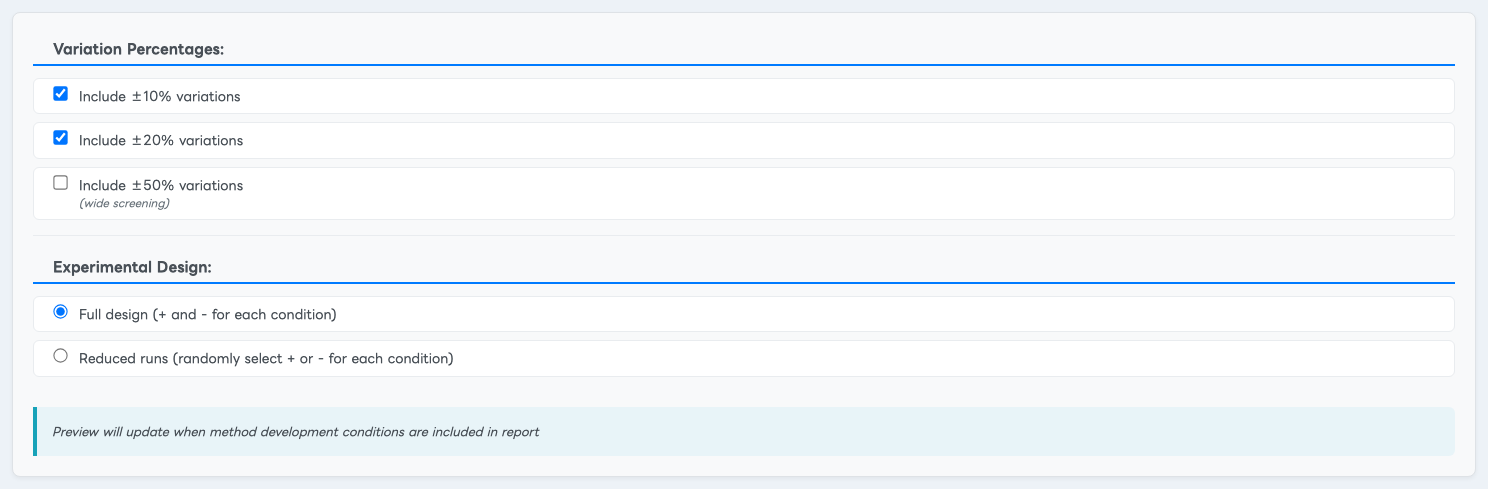
- Open Report Generation and select Method Development Conditions.
- For this worked example, retain ±10% and ±20% variations and the full design selection.
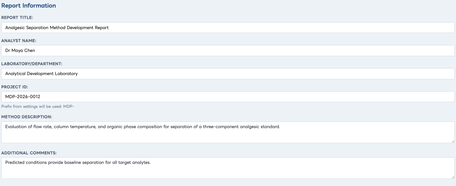
- Enter the round identifier and describe the failed critical pair in the report information.
- Select Generate Report.
Understand what was recommended
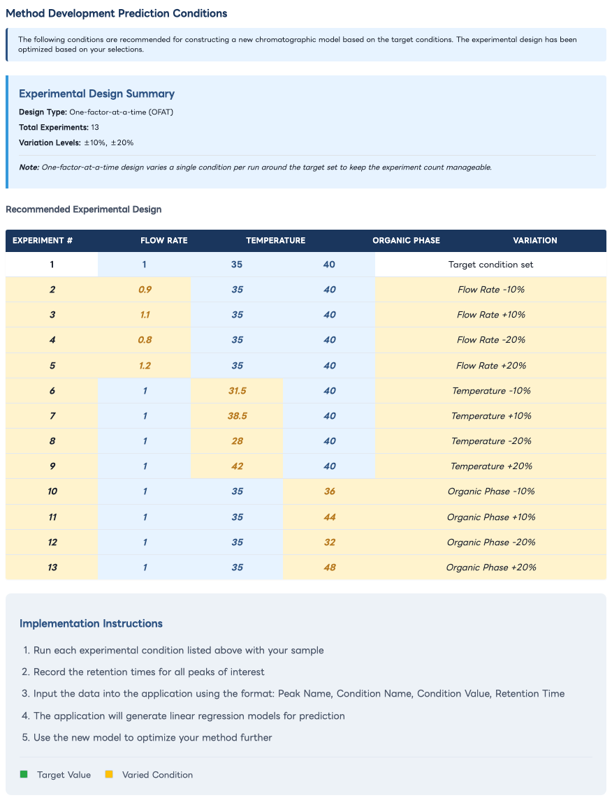
| Experiment | Flow Rate | Temperature | Organic Phase | Purpose |
|---|---|---|---|---|
| 1 | 1.0 | 35 | 40 | Confirm the centre / starting condition |
| 2–5 | 0.9, 1.1, 0.8, 1.2 | 35 | 40 | Measure Flow Rate response |
| 6–9 | 1.0 | 31.5, 38.5, 28, 42 | 40 | Measure Temperature response |
| 10–13 | 1.0 | 35 | 36, 44, 32, 48 | Measure Organic Phase response |
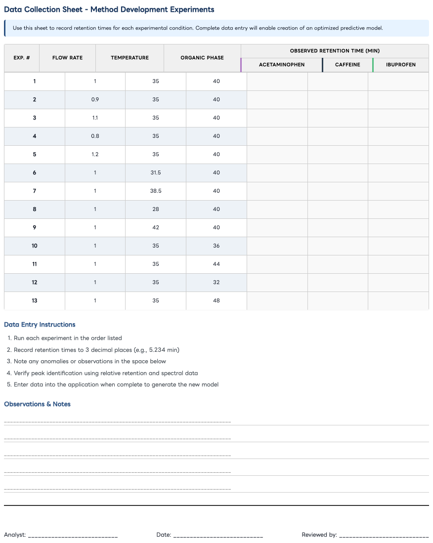
The report also creates a blank sheet with one row per condition and one RT column per named peak.
Run Round 1 and collect measured results
Goal: replace blank report cells with attributable laboratory observations.
- Run the 13 reviewed condition states in the approved sequence.
- At every condition, identify all three peaks and record their observed RTs.
- Record system-suitability results, anomalies, integrations, instrument/run identifiers, and any deviation from the proposed condition.
- Review the source data before transcribing it into ChromatographyForge.
The following values appear only after the fictional Round 1 experiments have been performed. They are tutorial results, not report predictions.
| Experiment | Flow | Temp. | Organic | Acetaminophen RT | Caffeine RT | Ibuprofen RT |
|---|---|---|---|---|---|---|
| 1 | 1.0 | 35 | 40 | 4.20 | 4.50 | 9.40 |
| 2 | 0.9 | 35 | 40 | 4.45 | 4.72 | 9.90 |
| 3 | 1.1 | 35 | 40 | 3.96 | 4.29 | 8.91 |
| 4 | 0.8 | 35 | 40 | 4.70 | 4.95 | 10.42 |
| 5 | 1.2 | 35 | 40 | 3.72 | 4.10 | 8.41 |
| 6 | 1.0 | 31.5 | 40 | 4.29 | 4.27 | 9.56 |
| 7 | 1.0 | 38.5 | 40 | 4.10 | 4.76 | 9.24 |
| 8 | 1.0 | 28 | 40 | 4.38 | 4.05 | 9.72 |
| 9 | 1.0 | 42 | 40 | 4.00 | 5.05 | 9.08 |
| 10 | 1.0 | 35 | 36 | 4.68 | 4.58 | 10.25 |
| 11 | 1.0 | 35 | 44 | 3.72 | 4.82 | 8.55 |
| 12 | 1.0 | 35 | 32 | 5.16 | 4.70 | 11.10 |
| 13 | 1.0 | 35 | 48 | 3.24 | 5.20 | 7.70 |
Enter Round 1 results and build the first model
Goal: transfer the measured experiment table into the application without changing its condition-first structure.
- Return to Quick Multi-Condition Entry.
- For Experiment 1, leave all conditions at baseline and enter the confirmed RT for each peak. If it is a genuine repeat, retain it as a replicate; investigate a material disagreement with the supplied starting run.
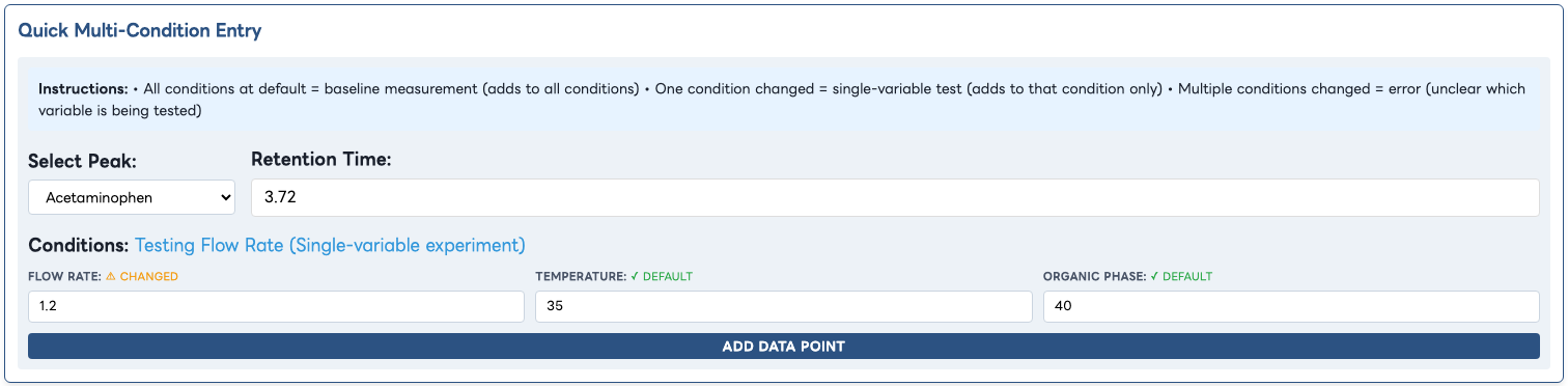
- For Experiment 2, set Flow Rate 0.9, add Acetaminophen 4.45, restore Flow Rate 0.9 after the form refresh, add Caffeine 4.72, then repeat for Ibuprofen 9.90.
- Continue experiment by experiment. Set one condition state, enter all three peak RTs, and only then move to the next row.
- Save the project after completing and checking each variable group.
Review the new evidence
Open each nested condition tab and reconcile the displayed points with the completed collection sheet. Then inspect slopes, R², missing values, and scientifically unexpected patterns.

- A high R² does not prove scientific validity or justify removing an inconvenient point.
- Order reversal at some tested states is a real development observation, not automatically a transcription error.
- Candidate modelling should normally stay within the measured Round 1 bounds.
Model and select a promising candidate
Goal: use the Round 1 model to choose the centre of the next experimental cycle.
Keep Initial Conditions at Flow Rate 1.0, Temperature 35, and Organic Phase 40. Test plausible Target Conditions one combination at a time. Watch the critical pair, elution order, and final-peak time together.
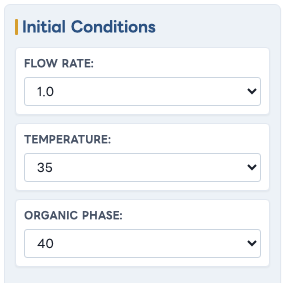
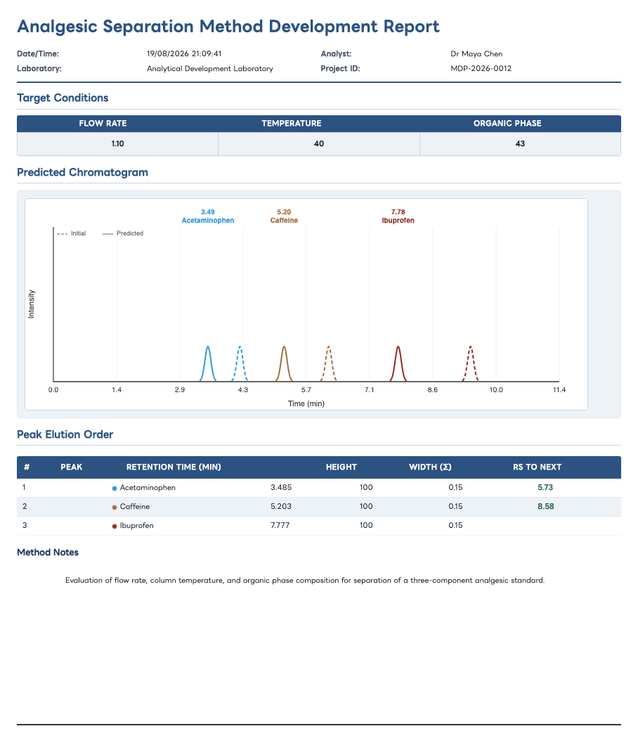
The tutorial selects Flow Rate 1.10, Temperature 40, and Organic Phase 45 as a Round 2 centre candidate. Every value lies inside the Round 1 measured range.

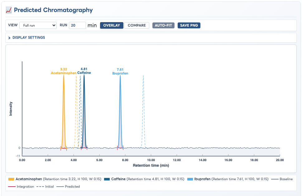

| Check | Initial model estimate | Round 2 centre prediction | Decision |
|---|---|---|---|
| Acetaminophen RT | 4.205 min | 3.224 min | Earlier |
| Caffeine RT | 4.510 min | 4.808 min | Moves away from Acetaminophen |
| Ibuprofen RT | 9.407 min | 7.615 min | Shorter predicted method |
| Critical-pair Rs | 1.02 | 5.28 | Promising enough to investigate |
The correct conclusion is “use this as the centre of Round 2”, not “method optimized.” It is a combined-condition prediction and still requires a new experiment set around it.
Generate Round 2 and repeat the model cycle
Goal: gather measured evidence around the promising candidate rather than accepting a single modeled point.
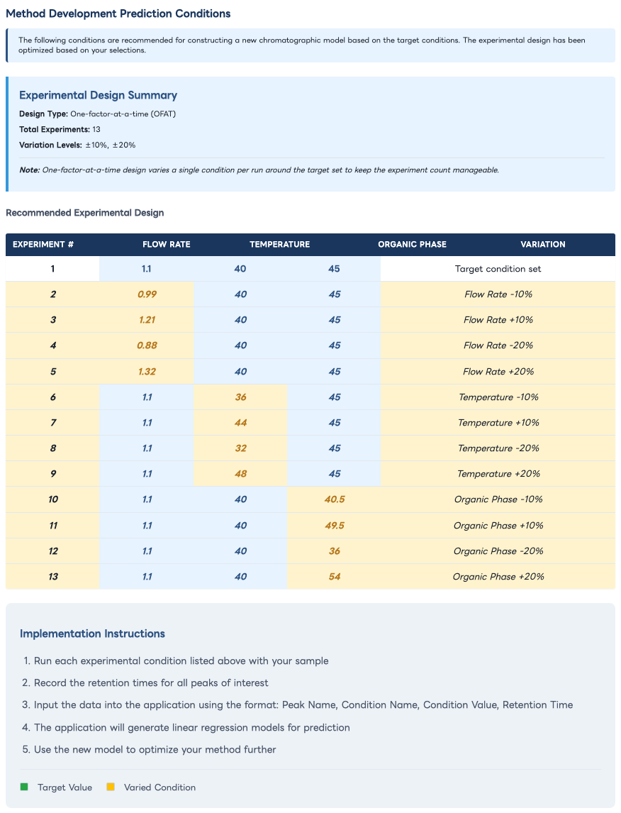
- Leave the Round 2 centre in Target Conditions: Flow Rate 1.10, Temperature 40, and Organic Phase 45.
- Open Report Generation, assign round identifier
MDP-2026-0012-R2, include Method Development Conditions, and generate the next plan. - Review each generated condition for scientific and equipment suitability.
Use a new model centre
Create a round-specific project such as Analgesic Development Round 2. Set its baselines to Flow Rate 1.10, Temperature 40, and Organic Phase 45, then create the same three peaks. This makes the Round 2 target condition the new baseline, so its report-generated rows can again be entered as baseline or single-variable experiments without ambiguity.
- Perform the approved Round 2 runs and record all three observed RTs at every condition.
- Enter those observations condition by condition in the Round 2 project.
- Review regressions, model another in-range candidate, and compare it with the Round 2 centre.
- If uncertainty remains or improvement continues, generate Round 3 around the new candidate and repeat.
Move from an optimised point to an operating range
Goal: show that acceptable performance is not confined to one exact set of numbers.
After one or more cycles, select the experimentally verified centre that best balances resolution, runtime, peak order, method practicality, and model quality. Then use the accumulated data to propose a preliminary operating range around it.
8.1 Propose a range from evidence
- For each condition, identify the interval actually covered by reliable results around the chosen centre.
- Use Target Conditions to inspect plausible low, centre, and high values inside those measured intervals.
- Record where predicted critical-pair Rs, elution order, and final-peak time continue to satisfy the development criteria.
- Narrow the proposal where the response changes quickly, model fit is weak, or an equipment/scientific constraint is approached.
8.2 Challenge the proposed boundaries
- Create a reviewed experimental plan that tests the proposed centre and appropriate range boundaries or combinations.
- Run the experiments and assess all method-specific criteria - not RT and Rs alone.
- Feed applicable single-variable results back into the model and compare observed versus predicted performance.
- If a boundary fails, contract the range or conduct another justified cycle. If performance is repeatable throughout the proposed region, document the evidence supporting the range.
| Operating-range question | Evidence expected |
|---|---|
| Does the critical pair remain acceptable? | Observed Rs meets the pre-defined criterion at challenged settings. |
| Is peak order stable? | No unacceptable reversal or co-elution across the tested region. |
| Is runtime practical? | The final peak and re-equilibration fit the method objective. |
| Is the response predictable? | Observed results are scientifically consistent with the fitted trends and investigated residuals. |
| Are interactions controlled? | Appropriate combined-condition or robustness experiments support the range where required. |
Report every cycle and retain the evidence
Goal: make the progression from failed initial method to proposed operating range understandable to another scientist.
- Use a round-specific title and ID for every report and project export.
- State the centre, generated conditions, safety-review changes, observed results, model assessment, candidate chosen, and reason for the next round.
- Include target conditions, chromatogram, elution order, resolution, statistics, method-development conditions, and raw points as required for technical review.
- Save active work to session and download the
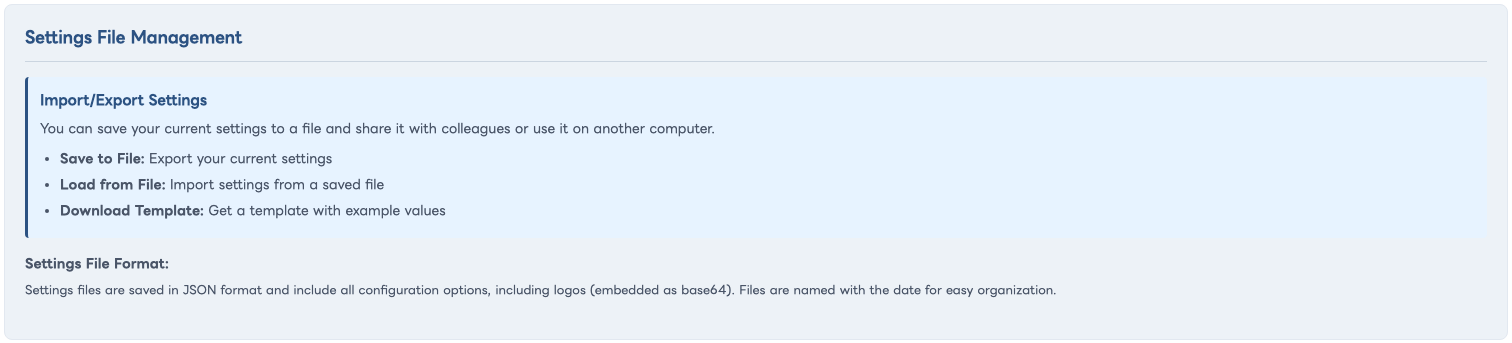
.hplcproject at meaningful milestones. - Retain report outputs, project exports, source chromatograms, completed collection sheets, anomalies, and the rationale linking one round to the next.
- Record the final optimised condition separately from the experimentally supported operating range and any remaining limitations.
Common beginner mistakes
| Mistake | Why it matters | Correct response |
|---|---|---|
| Entering imagined screening RTs before running experiments. | The model would be fitted to fiction. | Enter only the initial observed RTs, generate the plan, then wait for reviewed laboratory results. |
| Treating report recommendations as automatically approved. | Percentage variations can exceed safe or justified limits. | Apply the scientific and equipment safety gate to every generated row. |
| Optimizing after the initial single point. | There is no slope or response model yet. | Complete the first generated experiment round before selecting a candidate. |
| Entering report rows peak by peak. | This obscures which RTs came from the same run. | Set one condition state and add all observed peaks before moving to the next row. |
| Adding a combined candidate to the old model as a single-variable point. | The RT change cannot be attributed to one variable. | Use the candidate as the baseline of the next round-specific project. |
| Calling a strong prediction “optimized.” | Prediction is not experimental confirmation or robustness evidence. | Generate and execute the next round around the candidate. |
| Declaring an operating range from OFAT predictions alone. | Interactions and boundary robustness may be missed. | Challenge the proposed region with appropriate physical experiments. |
Plain-language glossary
| Term | Meaning in this tutorial |
|---|---|
| Initial condition | The one analytical method supplied at the start of Round 1. |
| Development centre | The method around which Report Generation calculates percentage variations. |
| Recommended condition | A proposed experiment produced by the report; it still requires safety and scientific review. |
| Observed RT | A retention time measured in a physical chromatographic run. |
| Predicted RT | A model estimate used to select an experiment, not an observed result. |
| OFAT | One-factor-at-a-time: one condition changes while all others remain at the current centre. |
| Candidate | A promising modeled condition chosen for the next experimental round. |
| Optimised condition | A condition selected after iterative modelling and experimental confirmation against the development goals. |
| Operating range | An experimentally supported region over which acceptable method performance is maintained. |
Where to go next
- Use ChromatographyForge UI Documentation for control-by-control instructions.
- Use ChromatographyForge Function Explanation for alternative entry routes and detailed operational behaviour.
- Repeat the tutorial with a different fictional critical pair, but begin with only the information actually available at that stage.
Tutorial version 2.1 • Revised August 19, 2026 • Updated to begin without pre-screened data and teach the complete iterative development cycle.